About:
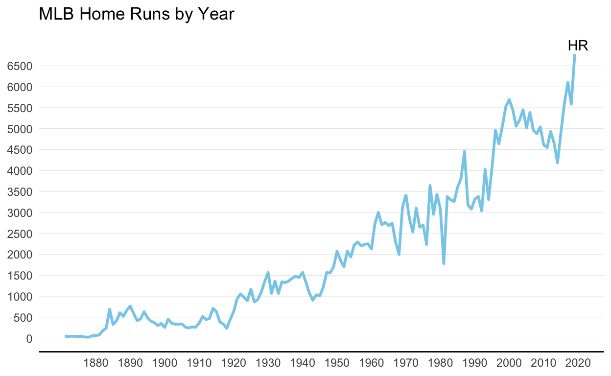
For this project I chose to replicate and re-design a visualization which shows how the number of MLB home runs per year has changed over time.
Link to the article containing the original graph and data:
Replica Graph:
Re-Designed Graph:
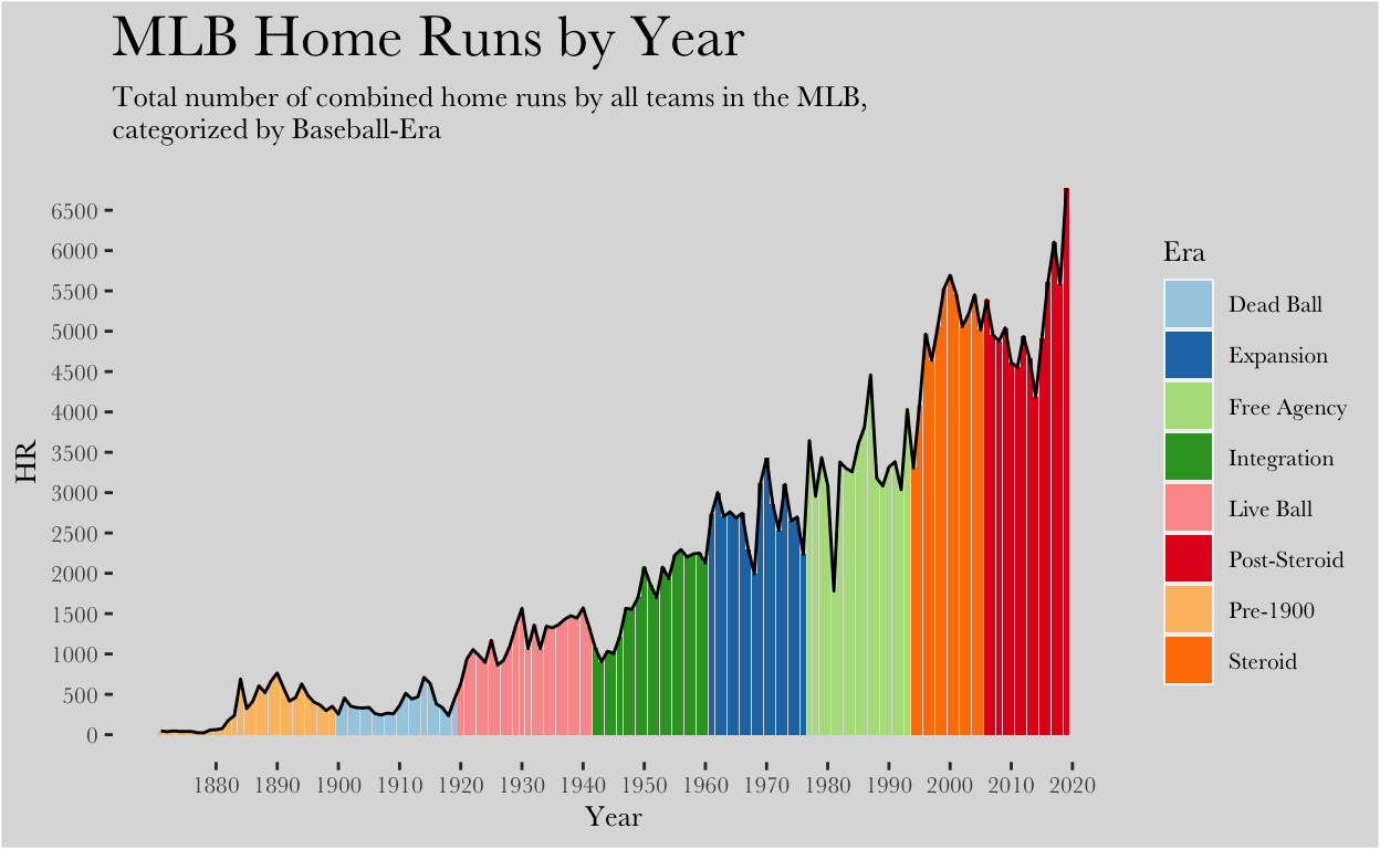
The original data set consisted of 2 variables (Year & Number of HRs) and 149 observations (1871-2020). I created a new variable, Era, which categorized what era of baseball each of the years fell into.
After I read the article the graph originated from, “A look into Major League Baseball’s massive home run splurge in 2019,” written by Ben Cooper, I learned that the main takeaway from the graph was intended to be the recent rise in home runs in the tail end of the Post-Steroid era. Avid baseball fans would know that after the MLB began testing for steroids, there was a long decrease in home runs, and bats did not fully come back alive until around 2016, and mostly 2019.
The original graph did display the increase; however, I created a new variable in the data set that accounted for Era to better explain the trend. I used the geom_col function because it allowed me to plot the year vs the number of home runs and fill the columns in by era. The reason I wanted to fill the columns by era was because it allows the reader to understand why there was a big drop in HRs followed by the highest peak in HRs ever recorded (the reason being because of the transition from the steroid to post-steroid eras). I also chose to use geom_line in addition to geom_col for the glow-up visualization. Since the columns are used to show the change in eras, the line is being used to show the trend between years. It is critical that visualizations must always be insightful, meaning they must help viewers make discoveries otherwise inaccessible. I believe that by creating an additional variable for the data set I made a more insightful graph for readers.
I also made some aesthetic changes to the graph, the first being the change in text. I chose a different custom font which I thought was more appealing and also increased the size of the title to make it easier for readers’ eyes. I also created a subtitle, to explain the variables in more detail. A change in background was also needed, since the stark white used in the original graph was too bright, so I replaced it with a subtle grey. Getting rid of the the axes was another change I made, for they were unnecessary for the point that was being proven.
After I read the article the graph originated from, “A look into Major League Baseball’s massive home run splurge in 2019,” written by Ben Cooper, I learned that the main takeaway from the graph was intended to be the recent rise in home runs in the tail end of the Post-Steroid era. Avid baseball fans would know that after the MLB began testing for steroids, there was a long decrease in home runs, and bats did not fully come back alive until around 2016, and mostly 2019.
The original graph did display the increase; however, I created a new variable in the data set that accounted for Era to better explain the trend. I used the geom_col function because it allowed me to plot the year vs the number of home runs and fill the columns in by era. The reason I wanted to fill the columns by era was because it allows the reader to understand why there was a big drop in HRs followed by the highest peak in HRs ever recorded (the reason being because of the transition from the steroid to post-steroid eras). I also chose to use geom_line in addition to geom_col for the glow-up visualization. Since the columns are used to show the change in eras, the line is being used to show the trend between years. It is critical that visualizations must always be insightful, meaning they must help viewers make discoveries otherwise inaccessible. I believe that by creating an additional variable for the data set I made a more insightful graph for readers.
I also made some aesthetic changes to the graph, the first being the change in text. I chose a different custom font which I thought was more appealing and also increased the size of the title to make it easier for readers’ eyes. I also created a subtitle, to explain the variables in more detail. A change in background was also needed, since the stark white used in the original graph was too bright, so I replaced it with a subtle grey. Getting rid of the the axes was another change I made, for they were unnecessary for the point that was being proven.
Appendix: Code
knitr::opts_chunk$set(echo = TRUE)
library(tidyverse)
#Load in data
library(readxl)
homeruns <- read_excel("HOMERUNS.xlsx")
#Create Replica Plot
library(tidyverse)
library(directlabels)
ggplot(data = homeruns, mapping = aes(x = Year, y = HR)) +
  geom_line(color = "skyblue", size = 1) +
  scale_x_continuous(breaks = seq(1880, 2020, 10)) +
  scale_y_continuous(breaks = seq(0,6500,500)) +
  labs(title = "MLB Home Runs by Year", size = 5) +
  theme_classic() +
  theme(
    panel.grid.major.x = element_blank(),
    panel.grid.major.y = element_line(size = .1, color = "lightgrey"),
    axis.title.y = element_blank(),
    axis.title.x = element_blank(),
    axis.ticks = element_blank(),
    axis.line.y = element_blank(),
  ) +
  annotate("text", x = 2020, y = 7000, label = "HR")
#create Glow-Up plot
library(extrafont)
ggplot(data = homeruns) +
  geom_col(mapping = aes(x = Year, y = HR, fill = Era)) +
  scale_fill_brewer(palette = "Paired") +
  geom_line(mapping = aes(x = Year, y = HR), color = "black") +
  scale_x_continuous(breaks = seq(1880, 2020, 10)) +
  scale_y_continuous(breaks = seq(0,6500,500)) +
  labs(
    title = "MLB Home Runs by Year",
    subtitle = "Total number of combined home runs by all teams in the MLB, \ncategorized by Baseball-Era"
    ) +
  theme(
    plot.background = element_rect(fill = "gainsboro"),
    panel.background = element_rect(fill = "gainsboro"),
    panel.grid.major = element_blank(),
    panel.grid.minor = element_blank(),
    text = element_text(family = "Baskerville", size = 10),
    plot.title = element_text(size = 20),
    legend.background = element_rect(fill = "gainsboro")
  )